By COMSOL, Inc.
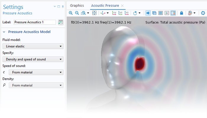
Simulation Software for Analyzing Acoustics and Vibrations Pressure Acoustics Modeling pressure acoustics is the most common use of the Acoustics Module. It includes capabilities for modeling effects such as the scattering, diffraction, emission, radiation, and transmission of sound. Simulations run in the frequency domain employ the Helmholtz equation, whereas in the time domain, the classical scalar wave equation is used. In the frequency domain, both FEM and BEM are available, as well as hybrid FEM–BEM. In the time domain, time implicit (FEM) as well as time explicit (dG-FEM) formulations are available. There are many options to account for boundaries in acoustics models. For instance, a boundary condition can be added for a wall, or an impedance condition can be added for a porous layer. Ports can be used to excite or absorb acoustic waves at the inlet and outlet of waveguide structures using multimode expansion. This applies to ducts, periodic structures, or boundary couplings to lumped acoustic models. Sources like prescribed acceleration, velocity, displacement, or pressure can be applied on exterior or interior boundaries. Furthermore, radiation or Floquet periodic boundary conditions can be used to model open or periodic boundaries. The dG-FEM time-domain-based formulation can be run on a GPU for increased performance in, for example, wave-based room acoustic simulation scenarios. Time-domain simulations are further enhanced with dedicated tools for including general frequency-dependent impedance conditions and porous material data. The Acoustics Module can also be used to model pipe acoustics, computing the acoustic pressure and velocity in flexible pipe systems. Applications include HVAC systems, large piping systems, and musical instrument components such as organ pipes. Electroacoustics: Speakers and Microphones When modeling speakers and microphones, it is essential to consider acoustic–structure interaction, where the fluid pressure causes a fluid load on the solid domain, and the structural acceleration affects the fluid domain as a normal acceleration across the fluid–solid boundary. The Acoustics Module includes a variety of acoustic–structure interaction capabilities. For modeling transducers of all sorts, the capabilities included in the Acoustics Module are readily combined with functionality from the AC/DC Module, the MEMS Module, or the Structural Mechanics Module to create fully coupled multiphysics FEM models. This includes detailed modeling of magnets and voice coils in loudspeaker drivers or the electrostatic forces in condenser microphones and electrostatic speakers. In electro-vibroacoustic (i.e., electro-mechanical-acoustic or electroacoustic) transducer systems, it is easy to use lumped circuit models or two-port representations to simplify the electric and mechanical components. Both approaches are solved with a full two-way coupling. There are also features for extracting the lumped representations from full FEM models. In addition, the (linear) small signal behavior and nonlinear large signal dynamics can be modeled and analyzed. In miniature transducer systems, like mobile devices, condenser microphones, and hearing aid receivers, the important damping due to the thermoviscous boundary layer losses is included. There is also extensive functionality for modeling piezoelectric transducers of all kinds. Microacoustics For an accurate microacoustic analysis of acoustic propagation in geometries with small dimensions, losses associated with viscosity and thermal conduction need to be accounted for, particularly the losses in the viscous and thermal boundary layers. These effects are automatically included when running a thermoviscous simulation using the Acoustics Module, and are important for vibroacoustics modeling in miniature electroacoustic transducers like microphones, mobile devices, hearing aids, and MEMS devices. In particular, a dedicated acoustic slip-wall condition exists for modeling MEMS devices with very small dimensions or operating at low ambient pressures. For detailed transducer modeling, there are built-in multiphysics couplings between structures and thermoviscous acoustic domains. The software accounts for additional thermoviscous acoustics physics effects, including the full transition from adiabatic to isothermal thermodynamic behavior at very low frequencies. Local nonlinear effects, such as vortex shedding in microspeaker ports or perforates, can be captured in the time domain with the addition of the nonlinear governing terms. Elastic Waves and Ultrasound in Solids The propagation of sound in solids happens through small-amplitude elastic oscillations of the solid's shape and structure. These elastic waves are transmitted to surrounding fluids as ordinary sound waves. The Acoustics Module can be used to model the propagation of elastic waves in solids and porous materials, for single-physics or multiphysics applications, such as vibration control, nondestructive testing (NDT), or mechanical feedback. Application areas range from micromechanical devices to seismic wave propagation. Elastic wave propagation over large domains containing many wavelengths is solved using a higher-order dG-FEM time-explicit method, and is multiphysics enabled for couplings with fluids as well as piezoelectric materials. The full structural dynamics formulation accounts for the effects of shear waves as well as pressure waves. The coupled propagation of elastic and pressure waves in porous materials solving Biot's equations (the mixed p-u formulation) can be modeled both for isotropic and anisotropic porous materials. Ultrasound in Fluids Acoustic signals with frequencies that are too high to be audible to humans are classified as ultrasound. In fluids, this implies that ultrasonic waves have a short wavelength. Simulating ultrasound in fluids requires computing the transient propagation of acoustic waves in fluids over large distances. With the software, this simulation can be done in two ways: modeling wave propagation that includes a background flow or modeling the effects of high-power nonlinear acoustics. It is possible to solve for transient linear acoustics in a simulation that contains many wavelengths in a stationary background flow by modeling the convected wave equation. Applications include flowmeters and exhaust systems. For high-power nonlinear acoustics applications, the software is able to capture progressive wave propagation phenomena where the cumulative nonlinear effects surpass the local nonlinear effects. This includes modeling the formation and propagation of shocks. Applications include biomedical applications such as ultrasonic imaging and high-intensity focused ultrasound (HIFU). For both options, there are multiphysics capabilities available for fully coupling a model with elastic waves in structures and/or with piezoelectric materials. Aeroacoustics Using the Acoustics Module, computational aeroacoustics (CAA) simulations can efficiently be run with a decoupled two-step approach. First, the background mean flow is identified using either the CFD Module, flow imported in the CGNS format, or a user-defined flow profile; then, the acoustic propagation is solved for. For convected acoustics simulations, several finite element formulations are available, including linearized Navier–Stokes, linearized Euler, and linearized potential flow aeroacoustics simulations. There is also support for computing acoustic variations in pressure, density, velocity, and temperature in the presence of any stationary isothermal or nonisothermal background mean flow. The formulations readily account for convection, damping, reflection, and diffraction of acoustic waves by the flow. There is also functionality for fluid–structure interaction (FSI) analyses in the frequency domain with predefined couplings to elastic structures. Additionally, tools are available for modal source decomposition and for conducting modal transmission loss simulations in the context of duct acoustics, such as those found in turbofan engines. Flow-induced noise can be included in a pressure acoustics analysis by the addition of aeroacoustic flow sources using Lighthill's acoustic analogy with input from a transient large eddy simulation (LES), detached eddy simulation (DES), or a transient Reynolds-averaged Navier–Stokes (RANS) shear stress transport (SST) model with scale-adaptive simulations (SST-SAS) with the CFD model. Room Acoustics The Acoustics Module offers an array of tools for analyzing the acoustics of rooms, such as concert halls, recording studios, and office spaces. For instance, there are geometrical acoustics formulations like ray tracing, wave-based methods, and hybrid approaches. Methods can be used together to perform a broadband analysis of a listening space. The geometrical acoustics capabilities of the Acoustics Module can be used to analyze high-frequency systems where the acoustic wavelength is smaller than the characteristic geometric features. There are two methods available for this type of analysis: ray acoustics and acoustic diffusion. For ray acoustics, the trajectories, phase, and intensity of acoustic rays can be computed. Additionally, impulse responses, energy and level decay curves, and the classical objective room acoustic metrics can be calculated. An atmosphere attenuation material model is available to include the attenuation in air as a function of temperature, pressure, and relative humidity. Additionally, the module features integrated couplings that enable transitioning from wave-based simulation results to ray tracing, enabling the realistic modeling of sources, such as loudspeakers, based on both near-field and far-field computations. For acoustic diffusion, there is functionality for determining the sound pressure level distribution in coupled rooms and the reverberation times at different locations. The acoustics are modeled in a simplified way using a diffusion equation for the acoustic energy density. This method is well suited for quick analyses inside buildings and other large structures. Wave-based simulations can be performed efficiently using the Pressure Acoustics, Time Explicit interface, which can be run on multiple GPUs for increased performance. This physics interface is supported for all license types when using a single GPU, but it requires a floating network license when using multiple GPUs. Realistic models can be set up using dedicated tools to include general frequency-dependent impedance conditions of walls and boundaries. Modal and time-harmonic simulations of rooms can be performed using the Pressure Acoustics, Frequency Domain interface. Dedicated iterative solvers exist for modeling large problems. Underwater Acoustics Underwater acoustics covers a wide range of applications, including transducer design, sonar technology, and noise propagation and mitigation. The Acoustics Module offers a comprehensive set of tools for modeling phenomena that span multiple length scales, frequency ranges, and multiphysics effects. Full electroacoustic modeling capabilities as well as piezoelectric multiphysics capabilities are essential for modeling underwater transducers. Sound propagation over large distances can be modeled with the Ray Acoustics interface. The rays can propagate in graded media (depth-dependent material properties), which is necessary in underwater acoustics applications, and a dedicated ocean attenuation material model is available to capture attenuation when propagating over large distances and at high frequencies. Additionally, the module features integrated couplings that make it possible to transition from wave-based simulation results to ray tracing, enabling the realistic modeling of sources, such as a vibrating ship hull or underwater piling noise, based on both near-field and far-field computations. Moreover, use of the BEM or Kirchhoff–Helmholtz formulation in the software is essential for analyzing the acoustic signature, like target strength (TS), of underwater objects. Acoustic Streaming With the Acoustics Module, it is possible to simulate acoustic streaming that describes the physical process where an acoustic field can induce movement in a fluid. The module contains multiphysics capabilities for coupling acoustics and fluid flow in order to model acoustic streaming phenomena for pressure and thermoviscous acoustics. Acoustic streaming is a nonlinear phenomenon that occurs due to the nonlinearity of the Navier–Stokes equations. The Acoustics Module computes the forces, stresses, and boundary slip velocities that the acoustic field induces in a fluid to generate the streaming flow field. This phenomena is used widely in biotech and semiconductor processing and is important in microfluidics and lab-on-a-chip systems for applications such as particle handling, the mixing of fluids, and microfluidic pumps. Features and Functionality in the Acoustics Module Built-In User Interfaces The Acoustics Module provides built-in interfaces covering all of the application areas listed above. These interfaces define sets of domain equations, boundary conditions, initial conditions, predefined meshes, predefined studies with solver settings, and predefined plots and derived values. All of the modeling steps performed with these interfaces occur within the COMSOL Multiphysics® environment. Meshing and solver settings are handled automatically by the software, with options for manual editing. The COMSOL Multiphysics® workflow for building acoustics models with the acoustics interfaces is the same as for building a model with any other physics interface. In this way, it is easy to incorporate multiple physics into one acoustics model, and there are several multiphysics interfaces built into the Acoustics Module and accessible when combining with other add-on modules from the COMSOL product suite. Pressure Acoustics Interfaces For modeling pressure acoustics, there are multiple interfaces where the sound field is represented by a scalar pressure variable. The general-purpose interfaces, based on FEM, include the capability of solving in both the frequency and time domain. For transient models, nonlinear effects can be included and are based on the Westervelt equation. To efficiently solve large radiation and scattering problems, frequency-domain BEM is available that couples seamlessly with both the acoustic and structural finite-element-based interfaces. To efficiently solve large transient models, a specialized interface based on the discontinuous Galerkin finite element method and a time-explicit solver is available. This interface can be coupled to the corresponding time-explicit interface for elastic and piezoelectric waves. For pure acoustic simulations, the time-explicit solver can run in a single- or multi-GPU setup for improved performance. Using the interface for boundary mode analysis, allows for studying propagating modes in the cross sections of waveguides and ducts. High-Frequency Pressure Acoustics Two highly specialized interfaces are available for quick high-frequency acoustics analysis in the frequency domain. These interfaces are based on computing the Kirchhoff–Helmholtz integral and include one interface for scattering analysis and another interface for radiation analysis. High-frequency acoustics analysis can be used as a first step before moving on to a more computationally demanding analysis based on FEM or BEM. Elastic Waves Interfaces The Acoustics Module includes interfaces for modeling the propagation of linear elastic waves in solids, porous, and piezoelectric materials. These interfaces readily couple to fluid domains using a set of built-in multiphysics couplings. The Solid Mechanics interfaces have the capability of representing full elastodynamics and can be used for modeling elastic waves in solids in both the frequency and time domain. A Port boundary condition is specifically implemented to model and handle various propagating modes in elastic waveguide structures. The poroelastic interfaces are used for modeling poroelastic waves in porous materials. These waves result from the complex two-way interaction between acoustic pressure variations in the saturating fluid and the elastic deformation of the solid porous matrix. The poroelastic interfaces solve Biot’s equations in the frequency domain and include loss mechanisms from viscous losses (Biot), for modeling rocks and soils, as well as thermal and viscous losses (Biot–Allard), for sound-absorbing materials in air. Models are available for materials with isotropic or anisotropic porous and structural properties, which are relevant in, for example, fibrous porous materials. Two interfaces, based on a time-explicit discontinuous Galerkin formulation, can be used for modeling linear elastic waves in solid and piezoelectric domains. These interfaces can be coupled and are suited for efficiently modeling domains with several wavelengths. A dedicated Fracture boundary condition can be used to model two solids with nonideal bonding, for example, if the goal is to simulate the acoustic response of a defect or a delamination zone. In addition, these interfaces can be coupled with the time-explicit interfaces for pressure acoustics and the convected wave equation. Aeroacoustics Interfaces For modeling detailed convected acoustics, or flow-borne noise, a number of aeroacoustics interfaces are available in both the frequency and time domain. These interfaces are used for simulating one-way interaction of a background fluid flow with an acoustic field. There are different physics interfaces that solve the governing equations under various physical approximations. The flow can either be computed in COMSOL using the CFD Module, or it can be imported using the CGNS file format. The Linearized Navier-Stokes interfaces are used for solving for the acoustic variations in pressure, velocity, and temperature. This formulation is the most detailed; it accounts for boundary layer losses as well as damping of acoustic waves in turbulent flow regions. The Linearized Euler interfaces are used for computing the acoustic variations in density, velocity, and pressure in the presence of a stationary background mean flow that is well approximated by an ideal gas flow. Special boundary mode interfaces are available for computing propagating and nonpropagating modes in waveguides and ducts in the presence of a background flow. Modal source decomposition and modal transmission loss simulations in duct acoustics, such as turbofan engines, can be achieved using the dedicated port conditions available with the Linearized Potential Flow interface. Liners are modeled using either the classical Ingard–Myers condition or the Brambley impedance condition that accounts for a finite flow boundary layer. Ray Acoustics and Acoustic Diffusion Interfaces The Ray Acoustics interface is available for running simulations in the high-frequency limit, where the acoustic wavelength is much smaller than the characteristic geometric features. In addition, for quick analyses, the Acoustic Diffusion interface is available for solving the acoustic diffusion equation, also known as energy finite elements. The interfaces for ray acoustics and the acoustic diffusion equation are suited for modeling acoustics in rooms and concert halls. The Ray Acoustics interface can also be used in outdoor or underwater scenarios. The Ray Acoustics interface is used to compute the trajectories, phase, and intensity of acoustic rays. It includes the capabilities of impulse response analysis, showing the level decay curves and computed objective room acoustic metrics, such as early decay time (EDT), T 60 values, etc. In addition, a set of dedicated features makes it easy to define sources and receivers with spatial directivity. There are also built-in couplings between wave-based simulations of various sources (such as transducers) and ray tracing, which simplify setting up realistic sources based on both the near-field and far-field results. Flow-Induced Noise Combining the Acoustics Module and the CFD Module results in a hybrid aeroacoustic (CAA) method for modeling flow-induced noise. The computational method is based on the FEM discretization of Lighthill's acoustic analogy (wave equation). This formulation of the equations ensures that any solid (fixed or vibrating) boundaries are implicitly taken into account. Windowing is available to truncate the source domain in space. The functionality relies on coupling an SST-SAS, LES, or DES fluid flow simulation, using the CFD Module, to an aeroacoustic flow source for pressure acoustics, available in the Acoustics Module. Finite Element and Boundary Element Methods Most interfaces in the Acoustics Module are based on different versions of FEM. Interfaces based on BEM are available as well, and can be seamlessly combined with FEM-based interfaces. Hybrid FEM–BEM is very efficient for modeling acoustic–structure interaction involving vibrating structures. Applications for hybrid FEM–BEM include complex geometries of transducers (piezo or electromagnetic) where FEM is used to model the transducer (and its interior) and BEM is used to model the exterior acoustics. A BEM-based interface can be used to replace an FEM-based radiation condition or PML, as well as the FEM-based exterior-field calculations. Boundary Conditions and Sources for Pressure Acoustics There is a large variety of boundary conditions available for pressure acoustics, including hard walls and conditions for applying sources. There are radiation, symmetry, periodic, and port conditions for modeling open boundaries. Impedance conditions include models for different parts of the human ear and human skin, simple RCL circuit models, and more. In the time domain, frequency-dependent impedance conditions can be set up using dedicated tools based on a partial fraction approximation of the data. The options for modeling idealized sources include built-in options for monopole, dipole, and quadrupole point sources. Extensive functionality is also provided for modeling waveguides using multimode expansions in combination with port boundary conditions. Port boundary conditions are used to excite or absorb acoustic waves at the inlets and outlets of ducts. A lumped port condition allows a waveguide to be coupled to a lumped acoustic representation, such as a lumped-element circuit or a transfer-matrix model. Periodic port conditions enable efficient simulation of absorption, transmission, and scattering in periodic structures, including diffusers and acoustic metamaterials. Acoustic–Structure Interaction Interfaces The interfaces for acoustic–structure interaction apply to phenomena where the fluid pressure causes a load on the solid domain and the structural acceleration affects the fluid domain across the fluid–solid boundary. This is also known as vibroacoustics. The interfaces include the capability of solving in either the frequency or the time domain. The solids included in the simulations can be isotropic, anisotropic, porous, or piezoelectric. When the Acoustics Module is combined with the Structural Mechanics Module, the structural side of an acoustic–structure coupling can additionally include structural shells or membranes. The Acoustics Module can be combined with the Multibody Dynamics Module in order to include the effects of multiple moving rigid or flexible parts connected through various types of joints. For more advanced options, the Acoustics Module can be combined with the AC/DC Module or MEMS Module to analyze fluid–structure interaction involving electric or magnetic forces, such as in cases where solids have electrostrictive or magnetostrictive material properties. Thermoviscous Acoustics Interfaces In order to accurately model acoustics in geometries with small dimensions, it is necessary to include thermal conduction effects and viscous losses explicitly in the governing equations. Near walls, there are viscous and thermal boundary layers. In these layers, viscous losses due to shear and thermal conduction become important because of large gradients. The interfaces for thermoviscous acoustics include the capability to simultaneously model the effects of pressure, particle velocity, and acoustic temperature oscillations. Thermoviscous acoustics is, for example, used when modeling the response of small transducers like microphones and receivers, also known as microacoustics. A multiphysics coupling with thermoelasticity physics allows for detailed modeling of damping in MEMS applications, including detailed thin-film damping. This functionality is further enhanced with a dedicated acoustic slip-wall condition necessary for systems with very small dimensions or operating at low ambient pressures. The condition should be used for the slip-flow regime when the Knudsen number is in the range of 0.001
The Microfluidics Module is designed specifically for handling momentum, heat, and mass transport with special considerations for fluid flow at the microscale. What Can Be Modeled with the Microfluidics Module: Perform various microfluidics analyses with the COMSOL® software. - Lab-on-a-Chip Devices: Compute the radial pressure distribution and flow rate through a rotating lab-on-a-chip platform. - Microfluidic Channels: Infuse and flush connected pieces of equipment with a fluid. - Micropumps: Model microfluidic systems with applications ranging from biological fluid handling to microelectronic cooling. - Micromixers: Simulate rapid mixing of different fluid streams. - Inkjet Printing: Model the fluid flow in an inkjet to predict optimal inkjet design. - Drug Delivery: Describe the operation of a drug delivery system. - Fuel Cells: Study proton exchange membrane (PEM) fuel cell designs and construction challenges. - Electrowetting Optical Devices: Modify a contact angle by changing the voltage applied to the conducting liquid. - Electrokinetic Valves: Analyze pressure-driven flow and electrophoresis in a 3D microchannel system. - Detection Tests: Study possible symmetries in the spreading of a liquid sample in a test strip. Features and Functionality in the Microfluidics Module: The capabilities of the Microfluidics Module can address multiple simulation problems. - Single-Phase Flow: The Fluid Flow interfaces use physical quantities, such as pressure and flow rate, and physical properties, such as viscosity and density, to define a fluid flow problem. The Laminar Flow interface covers incompressible and weakly compressible flows. This interface also allows for the simulation of non-Newtonian fluid flow. An interface for creeping flow is used when the Reynolds number is significantly smaller than one. This is often referred to as Stokes flow and is appropriate for use when viscous flow is dominant. It is usually applicable to microfluidic devices. - Three-Phase Flow: The Laminar Three-Phase Flow, Phase Field interface is designed to track the interfaces between three immiscible and incompressible fluids. This multiphysics interface couples a Laminar Flow interface to a Ternary Phase Field interface. The flow is assumed to be laminar; that is, the Reynolds number is low to moderate, and the density of each phase is constant. The interface solves the Navier–Stokes equations for the conservation of momentum as well as the continuity equation for the conservation of mass. The interface position is tracked by solving four additional transport equations, two for the phase field variables and two for the generalized chemical potentials. The movement of the surface is determined by the minimization of free energy. - Transport of Species: The Microfluidics Module provides a dedicated interface for transport of diluted species. It is used to simulate chemical species transport through diffusion, convection (when coupled with fluid flow), and migration in electric fields for mixtures where one component — a solvent — is present in excess (90 mol% or greater). It is typically employed to model the performance of mixers and Marangoni effects driven by concentration gradients. For modeling of chemical reactions in microfluidic devices, the Microfluidics Module can be combined with the Chemical Reaction Engineering Module, which also makes available transport of concentrated species with binary diffusion. - Electrokinetic Flow: When modeling the transport of diluted species, the electromigration of ions in a static electric field can be included according to the Nernst–Planck equation. Applications of this functionality include electrophoretic mobility and electroosmotic flow. The Microfluidics Module can be combined with the Chemical Reaction Engineering Module to access the Nernst–Planck interface and Electrophoretic Transport interface, which are dedicated to the modeling of electrolytes and can include the formulations of Poisson’s equation or the electroneutrality condition for the charge balance. The combination of Nernst–Planck and Poisson's equations can be used for modeling charged double layers and electroosmotic flow. - Two-Phase Flow: Three different methods are available in the Microfluidics Module for modeling two-phase flow: level set, phase field, and moving mesh methods. These are used to model two fluids separated by a moving fluid interface, where the interface is tracked in detail, including surface curvature and surface tension forces. The level set and phase field methods use a fixed background mesh and solve additional equations to track the interface location. The moving mesh method solves the flow equation on a moving mesh, and boundary conditions representing the fluid interface are directly applied at the surface. In this case, additional equations are solved for the mesh deformation by means of the arbitrary Lagrangian–Eulerian (ALE) method. All of these methods and their interfaces support both compressible and incompressible laminar flows, where one or both fluids can be non-Newtonian. - Porous Media Flow: Porous media flow can also occur in microscale geometries. When the pore size is in the micron range, the flow is often friction-dominated; in such cases, Darcy’s law can be used to solve the flow. The Microfluidics Module features a dedicated interface for porous media flow based on Darcy's law. In this case, shear stresses perpendicular to the flow are neglected. For intermediate flows, an interface for the Brinkman equations is available. This interface models flow through a porous medium where shear stresses cannot be neglected. There is support for both the Stokes–Brinkman formulation, suitable for very low flow velocities, and Forchheimer drag, which is used to account for effects at higher velocities. The fluid can either be incompressible or compressible, provided that the Mach number is less than 0.3. The formulation allows for free and porous media models, including porous media using the Brinkman equations or laminar flow. These interfaces are appropriate for microfluidic porous media flow. Example applications include paper microfluidics and transport in biological tissue. - Rarefied and Slip Flow: Rarefied gas flow occurs when the mean free path of the molecules becomes comparable with the length scale of the flow. The Knudsen number, Kn, characterizes the importance of rarefaction effects on the flow. As the gas becomes more rarefied (corresponding to how high the Knudsen number is), the Knudsen layer — which is present within one mean free path of the wall — begins to have a significant effect on the flow. For Knudsen numbers below 0.01, rarefaction can be neglected, and the laminar flow interfaces of the Microfluidics Module can be used with nonslip boundary conditions. For slightly rarefied gases (0.01 < Kn < 0.1), the Knudsen layer can be modeled by appropriate boundary conditions at the walls together with the continuum Navier–Stokes equations in the domain. In this instance, a Slip Flow interface is available in the Microfluidics Module. To model higher Knudsen numbers, the Molecular Flow Module is required. Expanded Modeling with the Microfluidics Module: As with the other products in the COMSOL product suite, when the Microfluidics Module is added to COMSOL Multiphysics®, the features and functionality are fully integrated into the modeling workflow and are ready to be used with other modules. For instance, the Microfluidics Module can be combined with the: - Heat Transfer Module to model thermal flows as well as conduction, natural and forced convection, Joule heating, thermophoresis, and Marangoni effects - AC/DC Module to study the effects of magnetophoresis and magnetohydrodynamics - Structural Mechanics Module to perform fluid–structure interaction simulations for fixed and deforming geometries with single-phase or multiphase flow - Chemical Reaction Engineering Module to model chemical reactions and transport of concentrated species and to access advanced capabilities for modeling transport of electrolytes and ions with electric fields as driving forces
CATEGORY
Model transport phenomena and chemical reactions relevant to various industries with the COMSOL® software. What Can Be Modeled with the Chemical Reaction Engineering Module: - Bulk Chemicals: Simulate space-dependent continuous stirred mixers and tank reactors for high flow rates. - Specialty Chemicals: Study reaction kinetics and mass transport to design processes for the fine chemicals industry, such as extraction and distillation processes. - Biotechnology and Pharmaceuticals: Optimize designs and processes for biotech and pharmaceutical applications by modeling the transport and reactions of drugs in tissue and across membranes. - Food Processing: Investigate heat transfer and reactions during pasteurization or study other processes in the food industry, such as drying, cooking, and fermentation. - Petrochemical: Model catalyst deactivation and pressure losses in packed bed reactors. - Environmental Technology: Investigate the elimination of pollutants in effluent streams using separation processes such as adsorption, membrane filtration, and crystallization. - Semiconductors: Study the rate of chemical vapor deposition (CVD) as a function of fluid flow and reaction kinetics in a CVD boat reactor. - Consumer Products: Design static mixers for laminar flow —such as mixers for epoxies, silicones, and acrylic resins — that achieve the desired emulsion properties. - Polymers: Study different aspects of polymer production processes, such as the dissolution of reactants, polymerization reactions, curing reactions, and filtration of the product stream. - Agricultural Chemicals: Investigate optimal process conditions and reactor design for the production of fertilizers, pesticides, and herbicides. Overview of the Modeling Strategy and Workflow: Realistic descriptions of reacting systems in scientific and engineering studies often need to incorporate both transport phenomena and chemical reactions. The Chemical Reaction Engineering Module includes features for following the typical workflow in chemical and chemical engineering investigations, which involves the following incremental steps: - Study reaction mechanisms in ideal, perfectly mixed systems - Calculate kinetic, thermodynamic, and transport properties - Extend the investigations to space-dependent system components that include: Transport of chemical species, Heat transfer, Fluid flow, Electrokinetic effects This workflow can be applied in many different fields that involve chemical reactions and for modeling at different scales, such as for the modeling of nanotechnology and microreactors as well as for environmental studies and geochemistry. The entire process, from defining models to the presentation of the results, is documented in the software for transparency and reproducibility. Features and Functionality in the Chemical Reaction Engineering Module: The Chemical Reaction Engineering Module provides a built-in workflow for simulating perfectly mixed systems in 0D followed by transport phenomena in 2D and 3D. Defining Reaction Kinetics: The first step in modeling any system is to establish the material balances. With the Reaction Engineering interface, chemical equations can be input in order to automatically obtain the material balance equations for the chemical species in the system and the energy balance equations for the system. When a reaction mechanism is added, the kinetic expressions as a function of the species concentrations are derived automatically from the mass action law for elementary steps. Users can also input their own analytical expressions for the reaction rate as a function of the species concentrations and temperature. The material balances and the reaction kinetic expressions give the ordinary differential equations that are formulated automatically by the software. For a perfectly mixed batch reactor, the solution to the equations gives the composition of the reacting mixture over time. Generating Space-Dependent Models: A working model for a perfectly mixed system can be used to automatically define material, energy, and momentum balances for space-dependent systems. The transport properties calculated in the Reaction Engineering interface (for example, heat capacity, thermal conductivity, viscosity, and binary diffusivity) automatically transfer to the physics interfaces for chemical species transport, heat transfer, and fluid flow. This functionality allows for refining kinetics and thermodynamics expressions of chemical reactions before moving to 2D, 2D axisymmetric, and 3D models. Chemical Species Transport: Modeling transport phenomena in reacting systems involves the description of the chemical species in so-called multicomponent transport models. The Chemical Reaction Engineering Module includes sophisticated models for multicomponent transport in the Transport of Concentrated Species interface, which offers the Maxwell–Stefan formulation and the mixture-averaged models for multicomponent transport. For diluted solutions, the Transport of Diluted Species interface is available, which treats cases where the interactions in the solution are dominated by solute–solvent interactions. The Dispersed Two-Phase Flow with Species Transport interface can be used to describe chemical species transfer between two immiscible fluid phases. The chemical species transport equations are also available for including Knudsen diffusion in, for example, porous media. The dusty gas diffusion model is also included. The formulation of the mass balance model as well as the transport properties can be obtained directly from chemical equations when generating a space-dependent model from the Reaction Engineering interface. Electrokinetic Effects: When modeling the transport of diluted or concentrated species, electric fields can be included as driving forces for transport for the modeling of electrolytes and ions. The Nernst-Planck and Electrophoretic Transport interfaces are dedicated to the modeling of electrolytes and can include the formulations of Poisson’s equation or the electroneutrality condition for the charge balance in the electrolyte. Applications of this functionality include electrokinetic valves, electroosmotic flow, and electrophoresis. Thermodynamic Properties Database: The Chemical Reaction Engineering Module contains a thermodynamic properties database, which can be used to calculate properties for gas mixtures, liquid mixtures, gas–liquid systems at equilibrium (flash calculations), liquid–liquid systems, and gas–liquid–liquid systems at equilibrium. There is a variety of thermodynamic models that can be used to calculate density, heat capacity, enthalpy of formation, enthalpy of reaction, viscosity, thermal conductivity, binary diffusivity, activity, and fugacity. Read more about this functionality on the Liquid & Gas Properties Module page, which is included in the Chemical Reaction Engineering Module. The thermodynamic properties database can be used to create a so-called property package for a specific reacting system by selecting the chemical species present in the system, the desired properties, and the thermodynamic model. When defining reaction mechanisms, the reactants and products can be matched with the chemical species in the property package defined by the thermodynamic properties database. This matching automatically links the functions and equations generated by the property package to the model of the reacting system. Parameter Estimation: Analysis of systems of chemical reactions and reaction mechanisms usually rely on parameter estimation of frequency factors, activation energies, and other parameters that may quantitatively describe experimental observations. The Chemical Reaction Engineering Module includes dedicated features for parameter estimation, designed to optimize these parameters using data from multiple experiments. The typical workflow for the estimation of model parameters is as follows: First, the model parameters to estimate (such as the rate constants) are selected, and the initial values and scales for the parameters are defined. Then, the experimental data is imported and data columns are correlated with model variables by entering the proper variable names or expressions. Next, an optimization method is chosen and computed. The progress of the optimization can be inspected during computation. Once the optimal parameter values have been found, the results can be compared with experimental measurements. Fluid Flow: The fluid flow functionality included the Chemical Reaction Engineering Module can handle laminar and porous media flow. Additionally, when combined with the CFD Module, there are ready-made couplings for the modeling of chemical species transfer in turbulent flow. The formulation of the fluid flow model as well as the viscosity and density can be obtained directly from chemical equations when generating a space-dependent model from the Reaction Engineering interface. Heat Transfer: The heat transfer functionality included in the Chemical Reaction Engineering Module can account for heat transfer by conduction, convection, and radiation. The radiation term is given by surface-to-ambient radiation, while the Heat Transfer Module is required for surface-to-surface radiation and radiation in participating media. The heat transfer capabilities of the Chemical Reaction Engineering Module include heat transfer in fluids, solids, and porous media. The formulation of the heat transfer model, as well as the thermodynamic and transport properties, can be obtained directly from chemical equations when generating a space-dependent model from the Reaction Engineering interface. Surface Reactions and Heterogeneous Catalysis: Surface reactions are typical for heterogeneous catalysis as well as for surface deposition processes such as chemical vapor deposition. They are found in the bulk chemicals industry, such as in the Haber–Bosch process for the production of ammonia and in microsensors for the detection of very low amounts of tracers that can adsorb on surfaces and be detected by, for example, a change in electrical properties. In transport-reaction models, surface reactions can be treated as boundary equations coupled to the boundary conditions for the transport and reaction equations in the bulk. This would be typical for models below or up to the microscopic scale. Alternatively, in porous media, these reactions are treated in a similar fashion as homogeneous reactions but include the specific surface area (area per unit volume of the porous material) and the effective transport properties. This would be typical for models both in the microscopic scale and the macroscopic scale — so-called multiscale models. The Chemical Reaction Engineering Module includes ready-made formulations for heterogeneous catalysis for surface reactions on boundary faces as well as surface reactions distributed over a homogenized porous catalyst. For porous catalysts, multiscale models are predefined to describe bimodal pore structures. Such structures may consist of microporous pellets packed to form a macroporous pellet bed.
CATEGORY
Model Low-Temperature Plasma Sources with the Plasma Module What Can Be Modeled with the Plasma Module Simulate the behavior of plasmas subject to a variety of electromagnetic excitations. Inductively Coupled Plasmas Investigate how power couples to the plasma in an ICP reactor. Capacitively Coupled Plasmas Model CCP reactors using a dedicated interface that directly solves the time-periodic steady state. Inductively Coupled Plasmas with RF Bias Investigate how an inductively coupled RF bias influences an ICP reactor. Nonisothermal Plasma Flow Couple a plasma model with fluid flow and heat transfer. Electron Cyclotron Resonance (ECR) Plasma Sources Couple a plasma model with magnetic fields and electromagnetic waves to model an ECR plasma source. Microwave-Excited Plasmas Investigate the effects of microwave heating in a plasma. Direct Current Discharges Simulate discharges sustained by a DC voltage or current. Corona Discharges Compute the spatial distribution of charged species in corona discharges. Electric Breakdown Detect if a high-voltage DC system can cause gas breakdown. Electrostatic Precipitators Track charged particle trajectories and compute the transmission probability of an electrostatic precipitator. Plasma Arcs Simulate the temperature distribution in a plasma arc and surrounding materials. ICP Torches Investigate the electrical and thermal characteristics of an ICP torch at atmospheric pressure. Plasma Global Models Model plasma reactors using global models for fast parameterizations and complex chemistries, including the Boltzmann equation. Electron Energy Distribution Functions (EEDFs) Compute EEDFs and obtain electron transport parameters and source terms for use in fluid plasma models. Optimization for Plasma Uniformity Optimize the coil design and positioning of an ICP reactor to obtain plasma uniformity. Ion Energy Distribution Function Compute the ion energy distribution function at surfaces. Etching and Deposition Simulate etching and growth rates along a surface. Features and Functionality in the Plasma Module The Plasma Module provides specialized tools for modeling low-temperature and thermal plasmas. Nonequilibrium Plasmas The Plasma Module provides built-in interfaces for modeling low-temperature plasma reactors that are sustained by a static or time-varying electric field. These interfaces each define sets of domain equations, boundary conditions, initial conditions, predefined meshes, and predefined studies with solver settings for steady and transient analyses, as well as predefined plots and derived values. Transport equations for all species (electrons, ions, and neutrals) are solved self-consistently with Poisson's equation. The electrons' mean energy equation can also be solved by modeling how the electrons gain energy from the electric field and lose energy in collisions with the background gas. Plasma Chemistry Reactions The plasma chemistry is extremely important for obtaining realistic simulation results. The Plasma Module can be used to define electron impact reactions, reactions between heavy species, and surface reactions. The plasma chemistry dictates how electrons lose or gain energy in collisions with the background gas. The Plasma Module offers dedicated features for modeling electron impact reactions that can result in ionization, excitation, and attachment. Electron impact reactions can be defined from cross-section data, and source terms can be obtained by suitable integration over electron energy distribution functions. Multiphysics Interface for Modeling ICP Reactors The Inductively Coupled Plasma multiphysics interface is used to study discharges that are sustained by induction currents. This multiphysics interface connects the plasma conductivity from the Plasma interface to the Magnetic Fields interface and couples the resulting electron heating due to the induction currents back to the Plasma interface. The magnetic field is solved for in the frequency domain and the plasma is solved for in the time domain. Multiphysics Interfaces for Modeling Equilibrium Discharges The Plasma Module includes interfaces for modeling plasmas in thermodynamic equilibrium. In thermodynamic equilibrium, electrons and heavy species have the same temperature, and the plasma can be characterized by a single temperature. To model plasmas in such conditions, the Plasma Module offers several Equilibrium Discharges interfaces that couple electromagnetics, fluid flow, and heat transfer, incorporating Lorentz force, electromotive force, enthalpy transport, Joule heating, and radiation loss. Multiphysics Interface for Modeling Microwave Plasmas The Microwave Plasma multiphysics interface is used to study discharges that are sustained by electromagnetic waves (wave-heated discharge). When this interface is selected, a Plasma interface and an Electromagnetic Waves interface are automatically generated, as well as multiphysics couplings. The Plasma Conductivity Coupling feature couples the plasma conductivity to the Electromagnetic Waves interface, and the Electron Heat Source feature couples the resulting electron heating back to the Plasma interface. The electromagnetic waves are solved for in the frequency domain and the plasma is solved for in the time domain. Boundary Conditions for Plasma–Surface Interactions As a part of the built-in interfaces within the Plasma Module, there are a variety of boundary conditions to describe how a plasma interacts with a surface. For example, electron density and energy fluxes at a surface are easily defined by applying the Wall feature. This feature introduces losses by transport to the electron transport equations. Additional flux sources can be included, such as secondary electron emission and generic electron fluxes at a surface. Fluxes of charged particles are automatically computed at electrodes and can be added to model external circuits. If a dielectric is in contact with the plasma, the surface charge accumulation can be computed from the fluxes of charged species at the surface. Surface Chemistry Reactions The Plasma Module includes a range of functionality for modeling etching and deposition processes in semiconductor fabrication processes. It solves plasma transport equations fully coupled with surface reaction kinetics, enabling the dynamic exchange of species between the surface and the gas phase. Surface site occupancy models can be used to accurately capture self-limiting reaction mechanisms. Furthermore, surface reaction rates can be specified with energy-dependent reaction yield models, facilitating detailed simulation of mechanisms such as ion-enhanced etching and energy-selective surface modifications. Multiphysics Interfaces for Modeling ICP Reactors with RF Bias The Inductively Coupled Plasma with RF Bias interface is used to study discharges that are sustained by induction currents and by an RF bias. This multiphysics interface connects the plasma conductivity from the Plasma, Time Periodic interface to the Magnetic Fields interface and couples the electron heating resulting from the induction currents back to the Plasma, Time Periodic interface. The magnetic field is solved for in the frequency domain and the plasma is solved for in the time domain. Multiphysics Interfaces for Modeling Fluid Flow and Heat Transfer of Background Gases The Nonisothermal Plasma Flow interfaces combine plasma, fluid flow, and heat transfer interfaces to model background gas flow and heating in a plasma reactor. The heat transfer in the materials surrounding a plasma can also be simulated. The Nonisothermal Plasma Flow multiphysics feature automatically computes the heat source resulting from plasma reactions and inputs it into heat transfer interfaces as a volume heat source. Fluid and thermodynamic properties like viscosity and thermal conductivity are computed in the Plasma interface and passed automatically to fluid flow and heat transfer interfaces. Physics Interface for Modeling CCP Reactors The Plasma Module includes a specialized numerical method for modeling CCP with significantly faster computation times than traditional methods. Instead of solving in the time domain, the periodic steady-state solution is computed by adding an extra dimension to the underlying mathematical equations. This extra dimensional equation represents one RF cycle and enforces periodic boundary conditions. This avoids having to solve for tens or hundreds of thousands of RF cycles, which typically takes a long time before the plasma reaches the periodic steady-state solution. This approach maintains all the nonlinearity of the model while dramatically reducing computation time.
CATEGORY
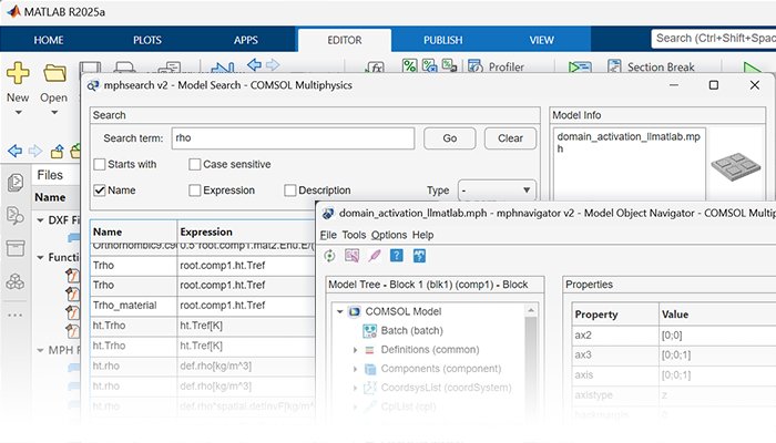
LiveLink™ for MATLAB® provides the necessary tools for maximizing the use of COMSOL Multiphysics® and MATLAB® in combination. Run Multiphysics Simulations from MATLAB® LiveLink™ for MATLAB® provides commands in the MATLAB® scripting language, sent from MATLAB® to COMSOL Multiphysics®, that initiate simulations in COMSOL Multiphysics®. This can be used for automating modeling steps as well as integrating COMSOL Multiphysics® models with calculations performed in MATLAB®. LiveLink™ for MATLAB® uses the COMSOL application programming interface (API), which has all the necessary functions and methods for implementing models from scratch or updating settings in existing models. All aspects of COMSOL Multiphysics® modeling can be controlled using MATLAB® through the API, which is tightly integrated with the MATLAB® environment. LiveLink™ for MATLAB® enables users to perform geometry and mesh operations, change physics settings, run parametric studies, control solvers, and postprocess the results. Results can be extracted as numerical data and MATLAB® figures. Utility Tools for Managing Models from MATLAB® All COMSOL® model settings are available from the command line in MATLAB®. To help get acquainted with the model data structure and the model settings, LiveLink™ for MATLAB® comes with two utility tools for navigating and searching the model contents: the Model Navigator and Model Search tools. The Model Navigator provides an overview of the model structure in a model tree together with the model settings and the commands that can be executed for each part of the model. Using this tool, it is easy to extract commands for setting and finding model properties to use in custom scripts. The Model Search tool will search the COMSOL Multiphysics® model from the MATLAB® interface, helping to find expressions and variables used in a model. Several filters and search settings are provided to narrow the search. Furthermore, a model from MATLAB® and the COMSOL Desktop® can be accessed simultaneously. This way, the workflow that is best suited for the task at hand can be used. It may be preferable to perform some tasks using the command line and scripting, while other tasks may be more convenient to perform using the COMSOL Multiphysics® user interface. Manage and Create Geometry Models and Meshes from MATLAB® Running COMSOL Multiphysics® from MATLAB® provides a lot of flexibility when handling geometry models and meshes. From MATLAB® programs and the MATLAB® command-line interface, it is possible to: - Generate geometry objects with inputs from MATLAB® - Import and export CAD models in a range of industry-leading file formats 1 - Run simulations based on imported CAD models - Create, import, and export surfaces on the STL, 3MF, and PLY file formats - Plot geometry objects in MATLAB® figures - Obtain geometry information for points, edges, surfaces, and domains, e.g., for adjacency, curvature, distances, etc. - Convert an image to a 2D geometry - Generate meshes - Plot meshes in MATLAB® figures - Retrieve mesh information such as mesh statistics and other mesh data - Import and export mesh data Call MATLAB® Functions from the COMSOL Desktop® LiveLink™ for MATLAB® provides a direct connection to MATLAB® while running COMSOL Multiphysics®. It is possible to call MATLAB® functions from the COMSOL Multiphysics® user interface to define material properties, boundary conditions, and more. These MATLAB® functions can be evaluated while the model is solving. Additionally, a COMSOL simulation app can contain MATLAB® calls, in which case MATLAB® will automatically start when called during runtime. Integrate with Existing MATLAB® Programs For MATLAB® users, COMSOL Multiphysics® simulations can easily be integrated into existing code bases. A model that has been set up in the COMSOL Multiphysics® user interface can be saved to an M-file. This M-file then contains COMSOL® API calls, in MATLAB® syntax, for running COMSOL Multiphysics® functionality. This provides a quick and convenient way of automatically generating COMSOL® modeling code, which can be used as a starting point for further integration into MATLAB® programs. Using the automatic code generation tools provides a quick way to learn the COMSOL® API for MATLAB®, which is included in LiveLink™ for MATLAB®. The COMSOL® API is easy to learn and has an intuitive structure similar to the steps used when setting up models in the COMSOL Multiphysics® user interface using the Model Builder. Existing code that is based on MATLAB® toolboxes or custom code integrates easily with COMSOL Multiphysics® simulations. Users can even call COMSOL Multiphysics® from user interfaces that have been created using MATLAB®. This makes it possible to, for example, use MATLAB® for data preparation and postprocessing and COMSOL Multiphysics® for structural, fluid, electromagnetics, or other physics or multiphysics modeling. Simulations can then be carried out using a mix of programs and models created with MATLAB®, COMSOL Multiphysics®, and even other tools. Generate Plots in MATLAB® and Extract Data from COMSOL Multiphysics® All COMSOL Multiphysics® plots can be recreated in MATLAB®. All plot types can be generated as regular MATLAB® plots and can be saved or exported and manipulated like any other MATLAB® plot. From MATLAB® programs, COMSOL Multiphysics® expressions can be evaluated either locally at a few points or for larger portions of a model, such as along the edges, on surfaces, or in volumes. Users can access the raw solution data or processed data based on arbitrary expressions, including maximum, minimum, average, and integral values. The COMSOL Multiphysics® unit handling is fully supported for any type of extracted data, which means that it is possible, for example, to use unit handling in custom programs for unit conversion. Any numerical data from COMSOL Multiphysics® simulations can be retrieved and assigned to MATLAB® variables for further analysis. Low-level information that is directly related to mesh and shape function data can be extracted, as well as sensitivities and time and spatial derivatives. 1. Requires one of the following add-on products: the CAD Import Module, the Design Module, LiveLink™ for SOLIDWORKS®, LiveLink™ for Inventor®, LiveLink™ for Solid Edge®, LiveLink™ for AutoCAD®, or LiveLink™ for Revit®
CATEGORY
